You're reading the documentation for a development version. For the latest released version, please have a look at master.

Procedure for Using HandEyeCalibration2DV02 Node

This node is one of the nodes used to perform robot-world 2D calibration for random bin picking. More specifically, this node calculates the 2D transformation between a robot virtual plane and the world (chessboard) where it is assumed that bin picking is performed on a 2D plane. In other words, this type of calibration can be used in scenarios where the picking height is constant. An overview of the calibration setup is shown below.

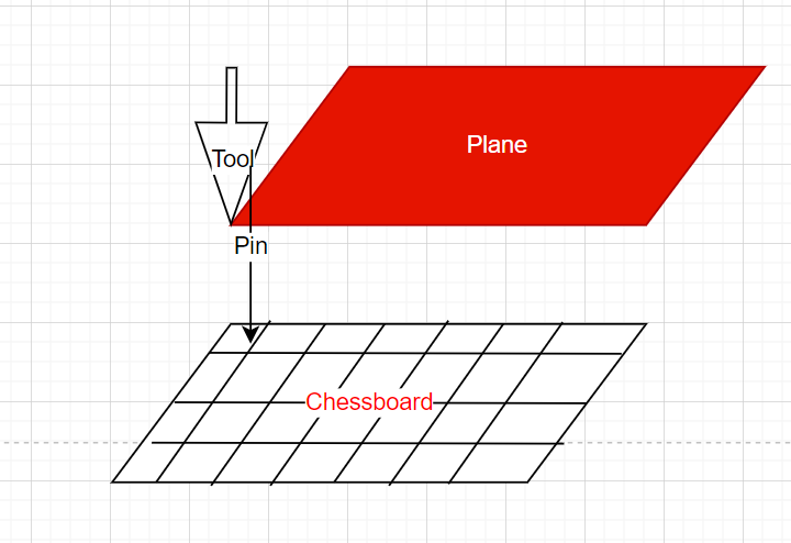
As shown above, this type of calibration requires you to place the chessboard on the object tray. We will refer to the chessboard coordinate system as the world coordinate system in the rest of this section. Also, a pin is attached to the robot arm and a robot virtual plane is defined using the robot pendent which should be parallel to the chessboard. Each robot type (robot brand) provides a way to define a virtual plane. Please refer to your robot manual for more details on how to do this.

In order to create this virtual plane, you need to define 3 different TCP positions. Then, the robot will automatically create a virtual plane with the Z axis directing upwards. Note that for the case of our calibration, we need to define the 3 TCP positions such that the pin touches the 3 corners of the chessboard on the tray.

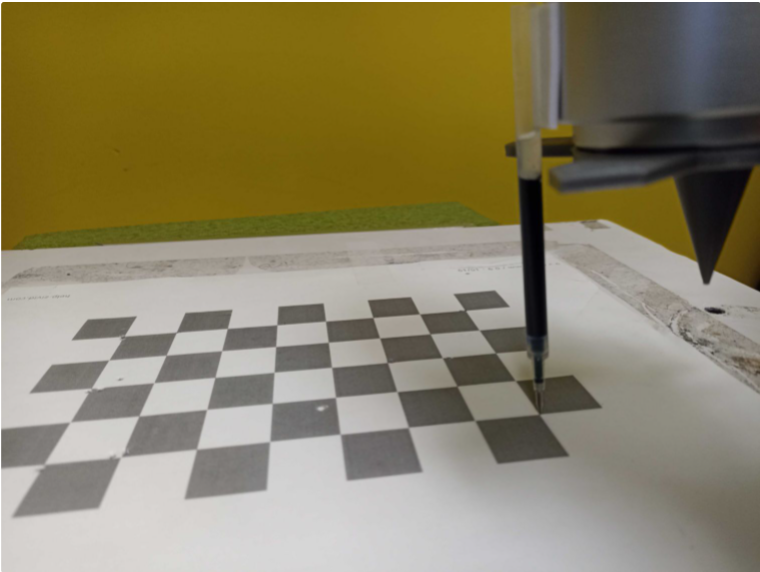
Once this virtual plane is created, We need to gather the calibration data needed. For this purpose, you need to move the the pin to corner points in the chessboard. The choice of the number of chessboard points to touch is arbitrary. However, our experiment with 12 points (3 rows and 4 columns) and using a row and column spacing of 2 squares is shown to give us a good and stable result. To better underhand this, as shown in the image below, you have to guide the robot to touch (nearly touch) the corner points of the chessboard in a zig zag pattern. Note that the distance between every two pin points in a row is called the row spacing value and the distance between every two pin points in a column is called the column spacing value (2 squares in this image). When touching the chessboard with the pin, the TCP value in the plane should have a Z value of near zero. Also, make sure the Rx and Ry values should be set to zero. Finally, use a variety of random rotation values for the Rz at each pin point on the chessboard to ensure a good calibration result. Once the robot pose (TCP in plane) for each pin position is collected, you need to save them for further use of the HandEyeCalibration2DV02 node. (Please refer to 2D picking flowchart template).

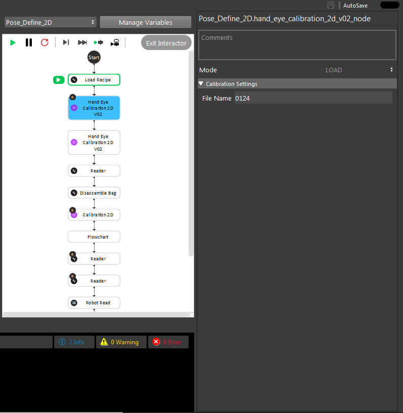
Now that the data has been collected, the HandEyeCalibration2DV02 node can be used to perform robot plane- world calibration. As mentioned before, the goal of this node is to find the 2D transformation between the robot plane and the world (chessboard). When adding the HandEyeCalibration2DV02 node, you will see that this node has three modes. The first mode is the accumulation mode which is used to load the calibration data (robot poses) needed for the calibration calculation.

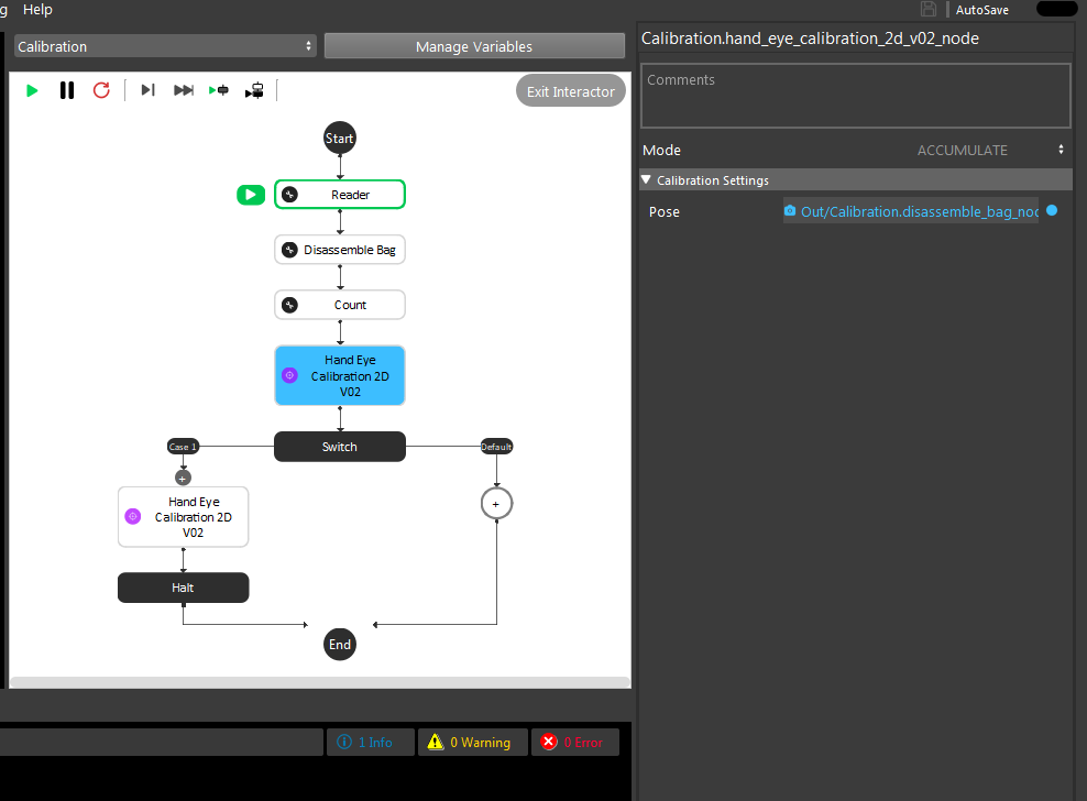
After accumulation, the next step is to perform the calibration computation and find the needed transformations. This is done using the final mode of HandEyeCalibration2DV02 node.

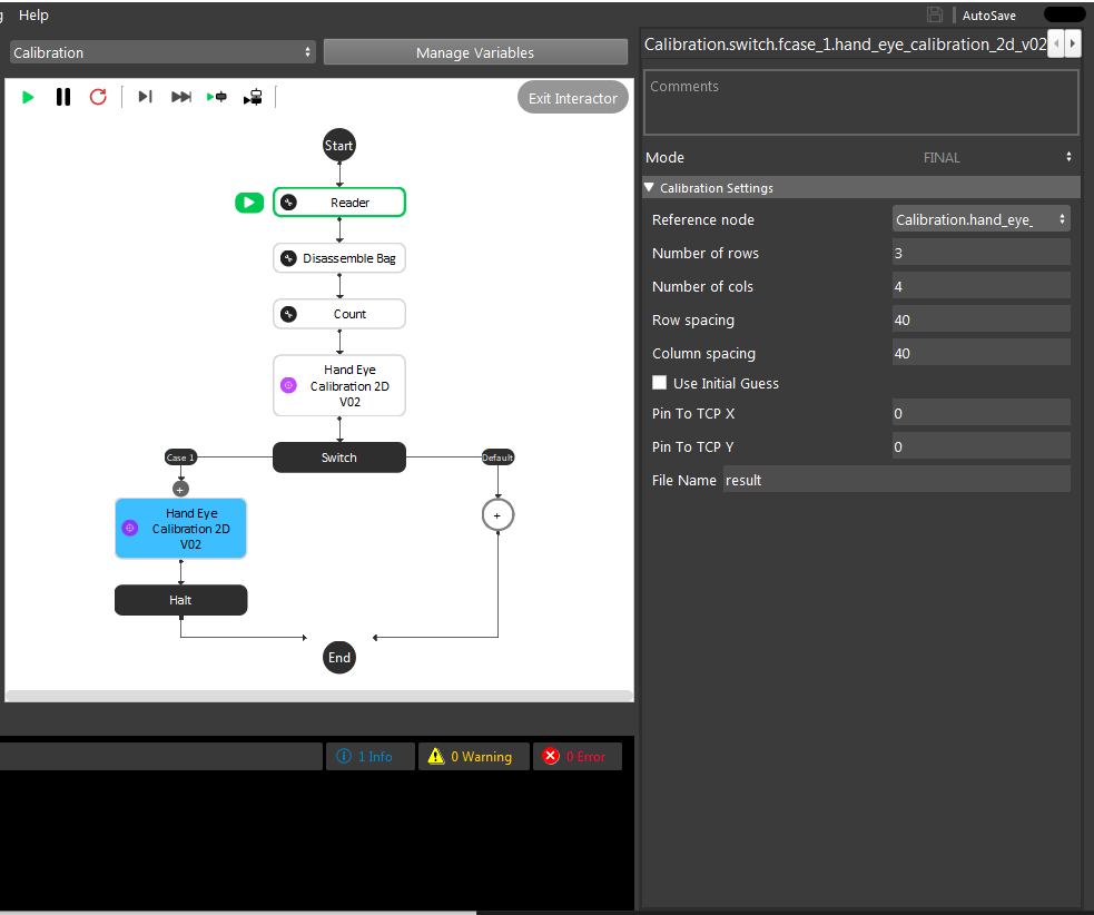
The output of the final mode is the 2D transformation of plane to world and world to plane alongside with the 2D translation of pin to TCP (saved in a 3D transformation format only including 2D components). The inputs of the node in the final mode include the reference node which is the reference accumulation node. Also, you have to specify the number of used row and columns for the pin points and distance between these points in each row and column (row spacing and column spacing). Also, you can specify an initial value for the translation of pin to TCP which is then used as an initialization for the optimization performed for calibration. Finally, the filename is the name of the file that the calibration results will be saved into. This then can be used to use the load mode to load the results later on without a need for performing the previous steps again as shown in the image below.